Simulation-free training of energy-based models

What are energy-based models and why are they interesting?

Energy-Based Models (EBMs) are a class of parametric unnormalised probabilistic models of the general form \(p_\text{ebm} \propto \exp(−U)\), originally inspired by statistical physics. In principle, any positive probability density can be modelled by an energy-function. By modelling the joint distribution of, for example, two inputs $x$ and $y$, energy-based models can be used to describe if $x, y$ are compatible with each other without specifying a functional relationship of the form $y = f(x)$. In consequence, many-to-many relationships or non-standard stochasticity of $y\mid x$ can be captured in a single probabilistic model. In general, energy-based models are useful tools in a wide range of applications such as conditional and compositional data generation, calibrated prediction, anomaly detection, or concept learning.

Why maximum likelihood estimation is challenging

We would like to estimate a neural data density using maximum likelihood estimation, i.e. maximising \(\mathbb E_{p_\text{data}(x)}[\log p_\theta(x)]\). Unfortunately, the maximum likelihood loss involves the intractable normalisation \(\log Z[U_\theta] = \log \int \exp(-U_\theta(x))\,\mathrm{d}x\). The most common workaround is contrastive divergence (CD) (Hinton, 2002), which approximates the gradient of the log-likelihood

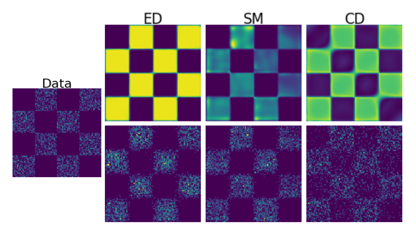
\[\nabla_\theta \log p_\theta(x) = \mathbb{E}_{p_\theta(y)}[\nabla_\theta E_\theta(y)] - \nabla_\theta E_\theta(x)\]

using short runs of a Markov chain Monte Carlo (MCMC) method to approximate the expectation under \(p_\theta\). For computational efficiency, the Markov chain is only run for a small number of steps. As a result, contrastive divergence does not learn the maximum-likelihood estimator and can produce malformed estimates of the energy function (Nijkamp et al., 2020). In particular, short-run MCMC leads to flattened energy landscapes that assign non-negligible probability mass outside the data support. This can, in part, be attributed to the fact that contrastive divergence is not the gradient of any fixed objective function (Sutskever & Tieleman, 2010), which severely limits the theoretical understanding of CD and has motivated various adjustments of the algorithm (Du et al., 2021).

Why tractable local losses can be insufficient

An alternative path consists in using local loss functions which are tractable, albeit costly. The most common one is score matching (Hyvärinen & Dayan, 2005): instead of comparing densities directly, one compares their score functions \(\nabla_x \log p_\text{data}\) and \(\nabla_x \log p_\theta\), which are by construction independent of the normalising constant. After an integration by parts, this yields the score matching loss

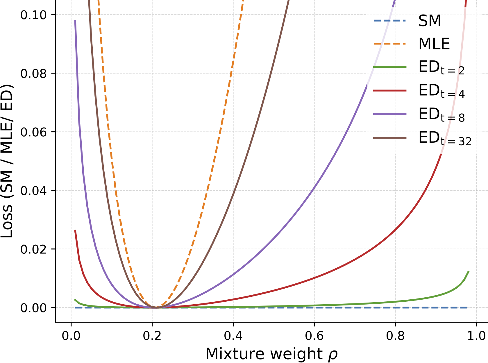
\[\text{SM}(p_\text{data}, U_\theta) = \mathbb{E}_{p_\text{data}(x)}\left[-\Delta_x U_\theta(x) + \frac{1}{2}\lvert\nabla_x U_\theta(x)\rvert^2\right]\,,\]

which can be estimated directly from data. However, since the score is a local quantity, score-based methods are nearsighted: in a mixture of well-separated distributions, the score matching loss decomposes into a sum of local objectives that only see each mode individually and are unable to resolve the mixture weights (Song & Ermon, 2019; Zhang et al., 2022).

On discrete data, where gradients are not available, people typically opt for pseudo-likelihood estimation. Pseudo-likelihood replaces the intractable joint likelihood with a product of conditional likelihoods \(\prod_i p_\theta(x_i \mid x_{\setminus i})\), each of which involves a normalisation over a single variable rather than the full configuration space. While this makes the objective tractable and consistent, pseudo-likelihood is also a local method: each conditional only captures the dependence of one variable on its neighbours, making it difficult to learn long-range structure in the distribution. Like score matching, it can therefore struggle to capture global features such as the relative weights of well-separated modes.

Local losses like score matching (SM) fail to capture global properties of a distribution such as mixture weights in a bimodal distribution. Maximum likelihood estimation (MLE) is generally preferable, but is often intractable. Energy Discrepancy (ED) let's us interpolate between them - the variance of the estimator decreases as ED approximates MLE with increasing $t$ parameter.

Energy Discrepancies: Broadening the design space for probabilistic self-supervised learning

Remarkably, we don’t have to decide between intractable losses like maximum likelihood estimation and local losses like score matching and pseudo-likelihood, but instead interpolate between them. The key idea is to compare the data distribution and the energy-based model via two contrasting energy contributions. Given a conditional perturbation distribution \(q(y \mid x)\), one defines the contrastive potential \(U_q(y) := -\log \int q(y \mid x)\exp(-U(x))\,\mathrm{d}x\) and the energy discrepancy as

\[\text{ED}_q(p_\text{data}, U) := \mathbb{E}_{p_\text{data}(x)}[U(x)] - \mathbb{E}_{p_\text{data}(x)}\mathbb{E}_{q(y \mid x)}[U_q(y)].\]

By definition, energy discrepancy only depends on the energy function and is independent of the scores or MCMC samples from the energy-based model. This definition is general: it applies on any measure space, including structured spaces like graphs or tabular data, provided the perturbation \(q\) involves some loss of information, i.e. \(x\) cannot be fully recovered from \(y \sim q(y \mid x)\). Under mild technical assumptions, energy discrepancy then has a global minimiser which is unique up to additive constants.

For Euclidean data with a Gaussian perturbation kernel \(\gamma_t(y-x) \propto \exp(-\lvert y-x\rvert^2/2t)\), the energy discrepancy can be expressed as a multi-noise-scale score matching loss, \(\text{ED}_{\gamma_t}(p_\text{data}, U) = \int_0^t \text{SM}(p_s, U_s)\,\mathrm{d}s\). This reveals that ED effectively integrates score matching objectives over a range of noise scales \([0,t]\), which alleviates the nearsightedness problem since the perturbed data distribution is more spread out. Furthermore, the Gaussian-based energy discrepancy converges to the loss of maximum likelihood estimation at a linear rate in time:

\[\lvert\text{ED}_{\gamma_t}(p_\text{data}, U) + \mathbb{E}_{p_\text{data}(x)}[\log p_\text{ebm}(x)] - c(t)\rvert \leq \frac{1}{2t}W_2^2(p_\text{data}, p_\text{ebm})\,,\]

where \(c(t)\) is independent of \(U\) and \(W_2\) denotes the Wasserstein distance. In other words, energy discrepancy interpolates between score matching for small \(t\) and maximum likelihood estimation for large \(t\), thus enjoying the attractive global properties of MLE while retaining a tractable, score-free loss. Similar statements can be obtained in the discrete case, too.

Energy Discrepancies in practice

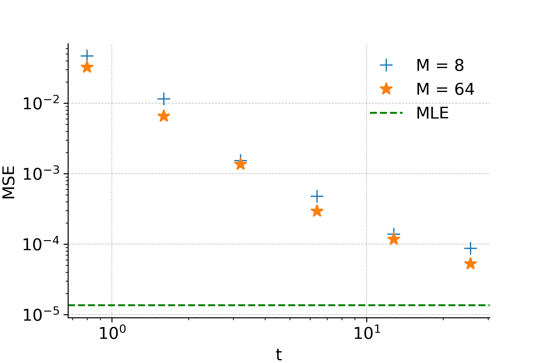
For Euclidean data \({x^i} \subset \mathbb{R}^d\) and a Gaussian perturbation kernel, energy discrepancy can be approximated from samples after noticing that the contrastive potential \(U_t\) of perturbed data can be written as an expectation \(U_t(x^i_t) = -\log \mathbb{E}_{\gamma_1(\xi')}[\exp(-U(x^i_t + \sqrt{t}\,\xi'))]\), which can be estimated by sampling \(\xi'^{i,j} \sim \mathcal{N}(0, I)\). However, a naive Monte Carlo approximation is biased due to the logarithm and prone to numerical instabilities. To stabilise training, we augment the estimate by an additional term \(w/M \cdot \exp(-U(x^i))\), called w-stabilisation, which provides a deterministic upper bound for the approximate contrastive potential and reduces the variance of the estimation. The full loss is then formed with tunable hyperparameters \(t\), \(M\), \(w\) as

\[\mathcal{L}_{t,M,w}(\theta) := \frac{1}{N}\sum_{i=1}^N \log\left(\frac{w}{M} + \frac{1}{M}\sum_{j=1}^M \exp\left(U_\theta(x^i) - U_\theta(x^i + \sqrt{t}\,\xi^i + \sqrt{t}\,\xi'^{i,j})\right)\right),\]

evaluated using the numerically stabilised logsumexp function. Each loss contribution only requires \(M\) forward evaluations of the energy function per data point in parallel — no spatial gradients and no MCMC sampling. In practice, the hyperparameter \(t\) controls the degree of nearsightedness (small \(t\) recovers score matching, large \(t\) approaches MLE), \(M\) controls the variance of the contrastive potential estimate, and \(w\) stabilises training by softly bounding the contrastive potential — larger \(w\) leads to flatter energy landscapes while smaller \(w\) yields steeper ones. Improved estimates of the energy discrepancy loss are possible, for example, through importance sampling.

The result is substantial improvements in training stability and estimation quality of energy-based models.

Citation

Energy Discrepancies: A Score-Independent Loss for Energy-Based Models

@article{schroder2023energy,
  title={Energy discrepancies: a score-independent loss for energy-based models},
  author={Schr{\"o}der, Tobias and Ou, Zijing and Lim, Jen and Li, Yingzhen and Vollmer, Sebastian and Duncan, Andrew},
  journal={Advances in Neural Information Processing Systems},
  volume={36},
  year={2023}
}

Energy-Based Modelling for Discrete and Mixed Data via Heat Equations on Structured Spaces

@article{schroder2024energy,
  title={Energy-based modelling for discrete and mixed data via heat equations on structured spaces},
  author={Schr{\"o}der, Tobias and Ou, Zijing and Li, Yingzhen and Duncan, Andrew},
  journal={Advances in Neural Information Processing Systems},
  volume={37},
  year={2024}
}